ملف:MultivariateNormal.png
حجم هذه المعاينة: 793 × 600 بكسل. البعد الآخر: 842 × 637 بكسل.
الملف الأصلي (842 × 637 بكسل حجم الملف: 159 كيلوبايت، نوع MIME: image/png)
وصف قصير
| ⧼wm-license-information-description⧽ |
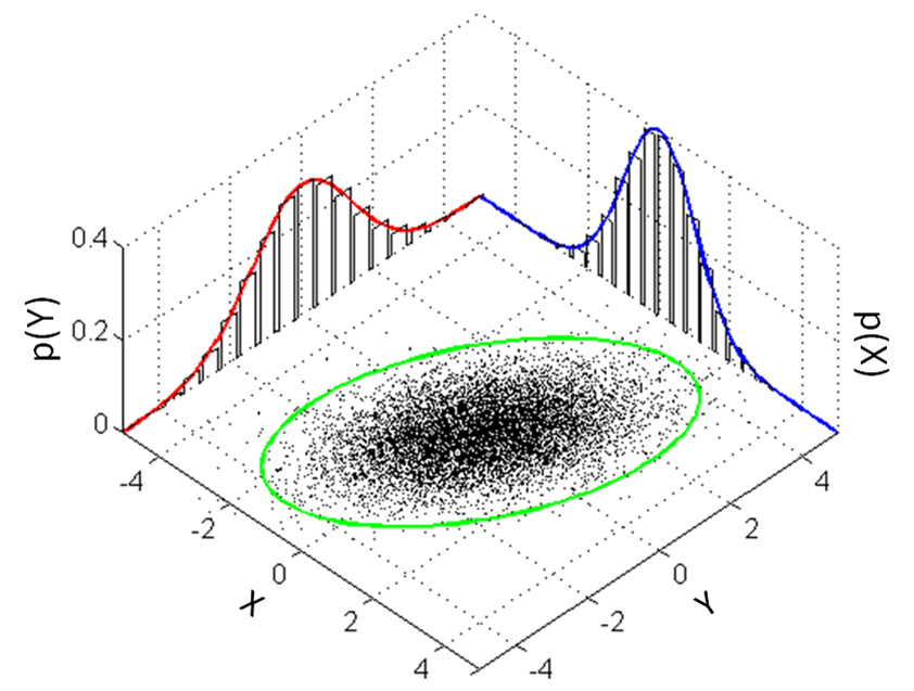
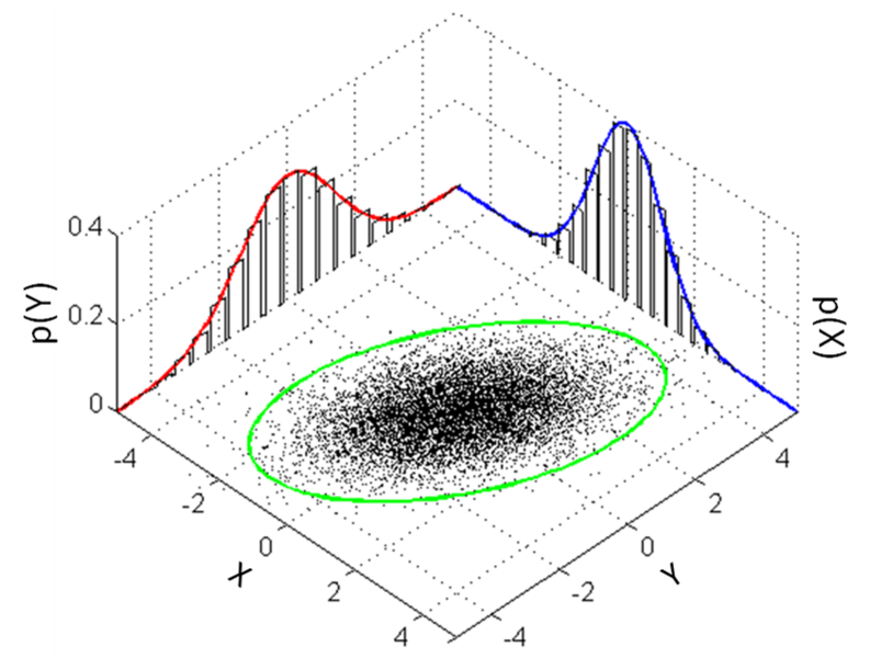
English: Illustration of a multivariate gaussian distribution and its marginals. Matlab code provided below.
|
| ⧼wm-license-information-date⧽ | 2013, {{time}} – invalid date format 28 (help) |
| ⧼wm-license-information-source⧽ | ⧼Wm-license-own-work⧽ |
| ⧼wm-license-information-author⧽ | Bscan |
%This script illustrates a multivariate Gaussian distribution and its
%marginal distributions

%This code is issued under the CC0 "license"

%Define limits of plotting
X = -5:0.1:5;
Y = -5:0.1:5;

%2-d Mean and covariance matrix
MeanVec = [0 0];
CovMatrix = [1 0.6; 0.6 2];

%Get the 1-d PDFs for the "walls"
Z_x = normpdf(X,MeanVec(1), sqrt(CovMatrix(1,1)));
Z_y = normpdf(Y,MeanVec(2), sqrt(CovMatrix(2,2)));

%Get the 2-d samples for the "floor"
Samples = mvnrnd(MeanVec, CovMatrix, 10000);

%Get the sigma ellipses by transform a circle by the cholesky decomp
L = chol(CovMatrix,'lower');
t = linspace(0,2*pi,100); %Our ellipse will have 100 points on it
C = [cos(t) ; sin(t)]; %A unit circle
E1 = 1*L*C; E2 = 2*L*C; E3 = 3*L*C; %Get the 1,2, and 3-sigma ellipses

figure; hold on;
%Plot the samples on the "floor"
plot3(Samples(:,1),Samples(:,2),zeros(size(Samples,1),1),'k.','MarkerSize',2)
%Plot the 1,2, and 3-sigma ellipses slightly above the floor
%plot3(E1(1,:), E1(2,:), 1e-3+zeros(1,size(E1,2)),'Color','g','LineWidth',2);
%plot3(E2(1,:), E2(2,:), 1e-3+zeros(1,size(E2,2)),'Color','g','LineWidth',2);
plot3(E3(1,:), E3(2,:), 1e-3+zeros(1,size(E3,2)),'Color','g','LineWidth',2);

%Plot the histograms on the walls from the data in the middle
[n_x, xout] = hist(Samples(:,1),20);%Creates 20 bars
n_x = n_x ./ ( sum(n_x) *(xout(2)-xout(1)));%Normalizes to be a pdf
[~,~,~,x_Pos,x_Height] = makebars(xout,n_x);%Creates the bar points
plot3(x_Pos, Y(end)*ones(size(x_Pos)),x_Height,'-k')

%Now plot the other histograms on the wall
[n_y, yout] = hist(Samples(:,2),20);
n_y = n_y ./ ( sum(n_y) *(yout(2)-yout(1)));
[~,~,~,y_Pos,y_Height] = makebars(yout,n_y);
plot3(X(1)*ones(size(y_Pos)),y_Pos, y_Height,'-k')

%Now plot the 1-d pdfs over the histograms
plot3(X, ones(size(X))*Y(end), Z_x,'-b','LineWidth',2);
plot3(ones(size(Y))*X(1), Y, Z_y,'-r','LineWidth',2);

%Make the figure look nice
grid on; view(45,55);
axis([X(1) X(end) Y(1) Y(end)])
ترخيص
تاريخ الملف
اضغط على زمن/تاريخ لرؤية الملف كما بدا في هذا الزمن.
| زمن/تاريخ | صورة مصغرة | الأبعاد | مستخدم | تعليق | |
|---|---|---|---|---|---|
| حالي | ★ مراجعة معتمدة 22:20، 6 نوفمبر 2023 | | 842 × 637 (159 كيلوبايت) | Pastakhov (نقاش | مساهمات) | Upload https://upload.wikimedia.org/wikipedia/commons/8/8e/MultivariateNormal.png |
لا يمكنك استبدال هذا الملف.
وصلات
لا يوجد صفحات تصل لهذه الصورة.